Executive Summary
The great disruption caused by COVID-19 has led to historic levels of economic volatility. As COVID-19 spread across the world, entire countries went into lockdown in an important attempt to curb the spread of the virus. Such lockdowns, however, brought economic activity to a standstill, as many businesses temporarily ceased operation or operated at a limited capacity. The halt and subsequent restart resulted in large swings in activity even within traditionally stable sectors of the economy. Further, the hole created by COVID-19 led to new outliers in many variables. These large deviations from historical trends will weigh on econometric models and alter analysts’ approach to forecasting. In a series of reports, we will discuss how this period may affect macroeconomic variables and econometric methods going forward as well as a framework for how to approach economic modeling in the post-COVID era.
In this first report, we discuss some potentially lasting effects of the recent swings in many macroeconomic variables. While the virus has injected new uncertainty in interpreting data, we advise continued caution as the economy slowly begins to dig itself out from the COVID-19 downturn. We identify issues that could arise as well as some data interpretation options to consider in the post-COVID era by drawing on some of our research after the Global Financial Crisis (GFC). Unprecedented economic volatility in the first half of 2020 may disrupt future seasonal adjustment processes and skew data. Further, some major variables may act differently in the post- COVID era, requiring adjustments in econometric models and a reconsideration of prior lead/lag relationships. It is also vital to not rely too heavily on one indicator or sector when assessing the health of the recovery.
Beware of Residual Seasonality
Widely followed macroeconomic data, such as Gross Domestic Product (GDP) and nonfarm payrolls are gathered by government agencies that provide a seasonal adjustment (SA) to the data.1 SA data can provide a clearer picture by removing fluctuations or seasonal patterns from the data that complicate time series analysis. SA also allows for a more accurate comparison of data over time. But, if SA data continue to exhibit a seasonal pattern within its data set, it could be due to residual seasonality.
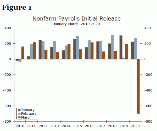
As we have highlighted previously, SA nonfarm payrolls data have demonstrated residual seasonality in the first quarter of every year since 2010. There is a “rogue” month each Q1 that is far above or below the other two months of the quarter (Figure 1). We have attributed the residual seasonality in nonfarm payrolls to GFC when there were 2.3 million jobs lost in the United States during the first quarter of 2009, which—prior to COVID-19—was the largest drop in a single quarter since 1945. This unprecedented decline likely disrupted the seasonal adjustment process resulting in residual seasonality lasting through 2019.2 We have also found evidence of residual seasonality in other variables such as GDP since the 2008 recession.3
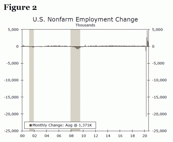
As seen in Figure 2 however, the 2.3 million jobs lost in Q1-2009 were dwarfed by the over 20 million jobs lost in just April 2020 (or over 13 million lost in Q2-2020). The virus-related hit to the jobs market today raises the natural question of how COVID-19 will disrupt the seasonal adjustment process going forward. Considering the virus impact on the labor market, the Department of Labor has already changed the way it adjusts initial jobless claims data for seasonality with its September 3 release. Instead of multiplying the unadjusted number by the seasonal factor, which is considered more accurate when the level of a series is generally steady, it has switched to an additive method. Given that the unadjusted level of claims is starkly higher than normal due to the pandemic and not usual seasonal factors, the multiplicative method has recently overstated the level of claims because August typically sees a below-average number of claims.
Other data collectors may soon follow suit. Almost every major macroeconomic variable (payrolls, GDP, retail sales, industrial production, etc.) experienced unprecedented swings in the first half of 2020 and those swings will likely disrupt pre-existing seasonal adjustment methods or perhaps result in residual seasonality in the post-COVID era. We think it will take some time to come up with an accurate set of seasonal factors to deal with the COVID-era swings. Although typically one set of seasonal factors are utilized for each variable, perhaps pre- and post-COVID seasonal factors will be developed to address concerns of residual seasonality stemming from COVID-19.4
Changing Behavior of Macroeconomic Variables5
Economic variables can also change behavior, or illustrate a noticeably different trend, after a recession. Being aware of possible changes is important because if a variable does not exhibit its pre-recession behavior, then econometricians may need to alter their models. A change in behavior in key variables can also affect expectations regarding the pace of recovery.
Virtually all sectors of the economy saw historically significant swings in 2008 and 2009, but only some have returned to their pre-crisis trend in the post-GFC era. The federal funds rate (FFR), for example, exhibited completely different behavior, as the extraordinary path of monetary policy during the crisis and subsequent recovery left the FFR far below its pre-recession peak throughout the post-GFC era. The unprecedented measures taken by the Federal Open Market Committee (FOMC) were necessary to stimulate the fledging recovery, but they undoubtedly changed how analysts utilize changes in the FFR in economic and financial models.
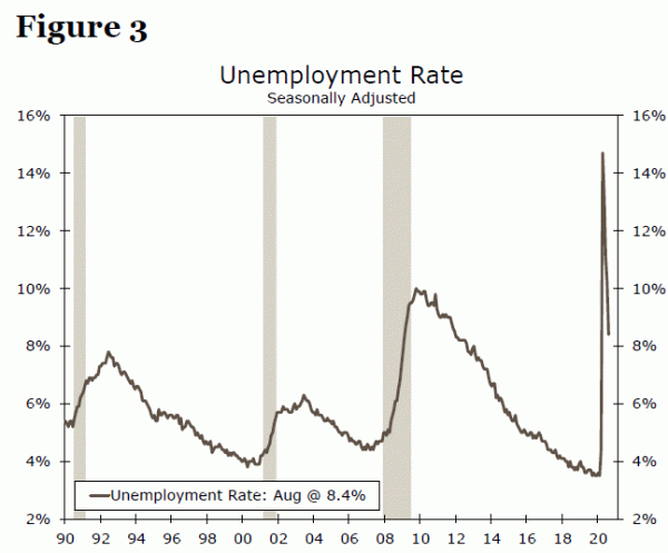
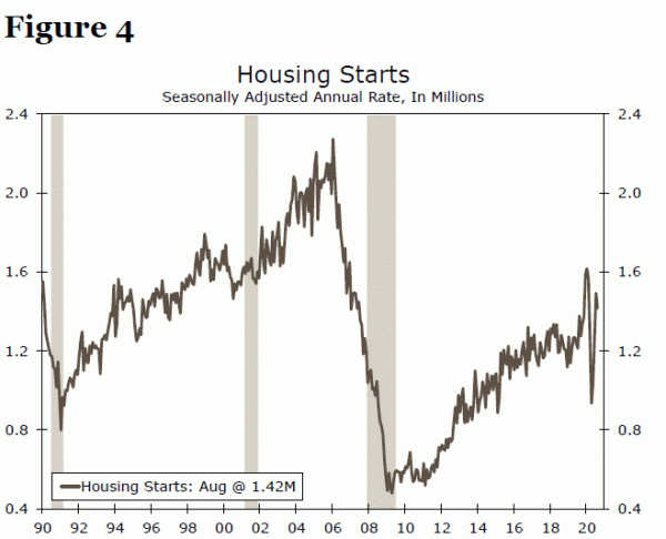
Of course, monetary policy was not the only area that the GFC affected in this manner. The unemployment rate (a proxy for the labor market) and housing starts (a proxy for the housing sector) were also altered by the crisis. The length of time for the peak unemployment rate to recover to its previous trough was 60 months after the 1991 recession and 43 months following the 2001 recession, but a whopping 91 months after the GFC (Figure 3). Housing starts also exhibited different behavior after the GFC. In fact, housing starts have still not reached their pre-recession level in the post-GFC era (Figure 4). Furthermore, housing starts stayed above one million units in the 1992-2007 period but dropped below this level from July 2008 until December 2012.
As the behavior of economic variables changes permanently, their dynamic with other variables (e.g. lead/lag relationships) need to be reconsidered. COVID-19 has already affected some of the traditional status of indicators. The Federal Reserve Bank of Philadelphia (Philly Fed), for example, produces a leading index for each state. However, the Philly Fed decided to suspend the release of the state leading indexes indefinitely, due to the impact of COVID-19 on initial jobless claims data, which is a component in the indices. The change in behavior of initial jobless claims had affected their estimation process.6
The Philly Fed’s state leading indices are unlikely to be the only victims of COVID-related volatility. As with the aftermath of the GFC, more variables will likely exhibit different behavior in the post- COVID era. This variation may even be more extreme given the volatility of the past few months. Moreover, the post-GFC era has some vital implications for those expecting the economy to get ‘back to normal,’ or those expecting a ‘normal’ pace of recovery. Expecting major sectors of the economy to bounce back to their pre-virus level or follow a similar recovery path as they did after previous recessions may misguide models, bias forecasts and ultimately lead to ineffective decisionmaking. Further, and perhaps more importantly, possible changes to macroeconomic variables emphasize the need to pair quantitative econometric analysis with qualitative understandings.
Don’t Underestimate the Power of an Index
With that in mind, it is important not to rely on any one variable to measure the health of a sector. Different variables from a sector can send mixed signals and cause serious challenges for decision makers. The labor market recovery in the post-GFC era is a good example. The economic expansion following the GFC is widely considered a “jobless” recovery. However, nonfarm payroll growth was healthy, while initial jobless claims and the unemployment rate were falling (2010-2012). Still, analysts were puzzled by weak wage growth and low labor force participation. A common question among labor market observers was the degree of slack in the labor market. Obviously, the answer depended on what information an analyst employed (payrolls or wage growth).
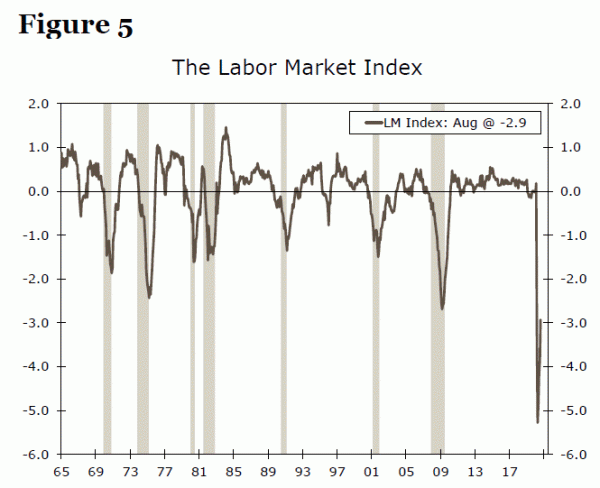
One way to avoid or perhaps placate mixed signals is to employ an index approach. For example, we previously developed the Labor Market Index (LMI), which consists of six variables and captures the supply and demand dynamics of the U.S. labor market (Figure 5).7 The LMI thereby provides a more accurate and holistic picture of the labor market versus analyzing just one variable. An ideal recovery would be evident across all major labor market indicators, not just one or two, but an index-based approach can ensure all variables are considered.
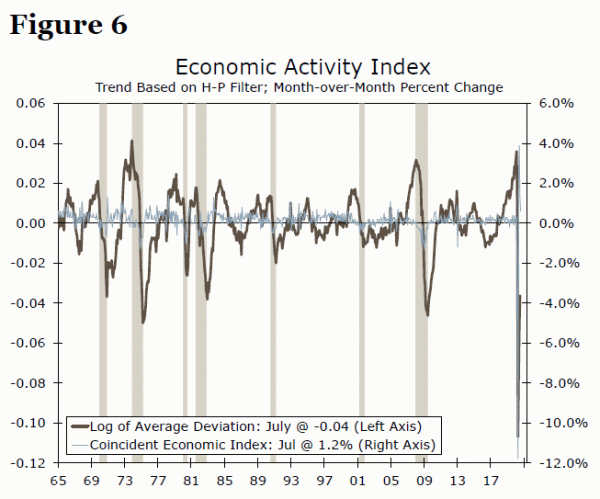
Unprecedented volatility from COVID-19 can also blur the picture of a sector’s health. One practical approach to handling such volatility is to apply the Hodrick-Prescott (H-P) filter on the series to evaluate if the variable is above or below its trend.8 The major benefit of the H-P filter is that it can be adjusted to handle volatility. For example, we utilize this technique to gauge the current state of the economy by applying the H-P filter on the four series (nonfarm payrolls, industrial production, personal income less transfer payments and manufacturing and trade sales) of the Conference Board’s Coincident Economic Index (CEI). As seen in Figure 6, the index is smoothed but still shows the severity of the current downturn. Utilizing the H-P filter to estimate the pace of recovery for desired sectors should prove useful in the post-COVID era as it will help parse through month-to-month volatility.
Don’t Forget Animal Spirits
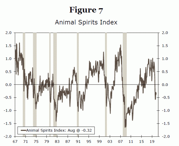
Finally, referencing a measure of animal spirits—what Keynes once remarked as one of the key factors behind fluctuations in the economy—may help estimate the extent of the damages from COVID-19 and the expected pace of recovery. We previously quantified animal spirits by constructing the Animal Spirits Index (ASI), which includes five variables that capture actions of major economic agents and represent major sectors.9 In reference to Figure 7, the largest negative ASI value is -1.65 (October 2008), which indicates the severity of the GFC. Furthermore, the ASI stayed negative (indicating pessimism) until January 2014, which is consistent with the slow recovery from the GFC.
At the onset of the COVID crisis in March, the ASI fell sharply and has remained negative through July. It is important to note that some of the major macroeconomic data (retail sales, ISM indices, etc.) are already showing signs of recovery. However, the past five months of negative ASI values indicate an underlying lack of confidence in the current recovery. Based on the historical performance of the ASI, we suggest analysts await continuous momentum in the ASI before declaring a full recovery is underway. Therefore, the ASI should remain a useful indicator to gauge the state of the economy in the post-COVID era.
Conclusion
We want to conclude by emphasizing the potential data issues arising from COVID-related volatility. First, being aware of residual seasonality is important for analysts as they interpret data in the fledging recovery. Second, re-evaluating macroeconomic variable behavior and adjusting model inputs in the post-COVID era may be crucial. Third, with certain variables being vulnerable to disruptions in their seasonal adjustment or a change in behavior, it is important to not rely too heavily on one single indicator when assessing the health of a sector. Finally, analysts should also reference a measure of animal spirits for a sustained pick-up in expectations when gauging the recovery.
All of the highlighted potential issues are known to us today, but they were unknown to most analysts in the early-phase of the post-GFC era. This is all to say, even if we are prepared for similar changes in regards to macroeconomic variables in the post-COVID era as we saw after the 2007-09 recession, it is likely we will face some unknown modeling difficulties in the years ahead. A practical approach to prepare for such unknown outcomes is to acknowledge their possibility and to reevaluate or test the behavior of data, which we have suggested throughout this report. By testing, an analyst would find signs of a change in a variable’s behavior early on, which could help redesign models’ accordingly.
In the next part in this series, we will delve into new modeling and estimation techniques that we recommend be utilized in the post-COVID era.
1 Some key private-sector data are also seasonally adjusted, such as the Institute for Supply Management Manufacturing and Services indices. But, not all data are seasonally adjusted and seasonal adjustment versus non-seasonal adjustment is an important distinction when analyzing data.
2 As shown in Figure 1, the January 2019 payrolls number is far from both February (absolute difference between Jan. and Feb. was 284K) and March (the difference between Jan. and March was 144K).
3 Q1 GDP tends to be weaker than other quarters in the 2010-2016 period, which is also attributed to residual seasonality from the GFC.
4 It may take a while to find a reliable method to seasonally adjust the COVID-era data. A permanent solution is beyond the scope of this report and we leave that question for future research.
5 This section builds on a previous report; “COVID-19: A Black Swan or a Group of Black Swans?“
6 For more detail, please see, “State Leading Indexes.”
7 The six LMI variables are: Nonfarm payrolls, labor force participation rate, U3 unemployment rate, average hourly earnings, initial claims for unemployment insurance and average weekly hours.
8 An H-P filter-based index is typically good to examine where a variable is at a particular point of time relative to its long-run trend as it estimates a long-run trend and separates cycles from the trend. For more detail on the H-P filter, please see Silvia et al. Economic and Business Forecasting. (2014).
9 The five ASI variables are: S&P 500 Index, Conference Board’s consumer confidence index, yield spread between the 10-year U.S. Treasury and federal funds rate, VIX index and economic policy uncertainty index. A dynamic factor modeling (DFM) approach is used in constructing the ASI. An ASI value above zero indicates optimism and a value below zero indicates pessimism. The DFM approach extracts information from each point of time and thus the current month value would be relative to the last month index value.

