Sample Category Title

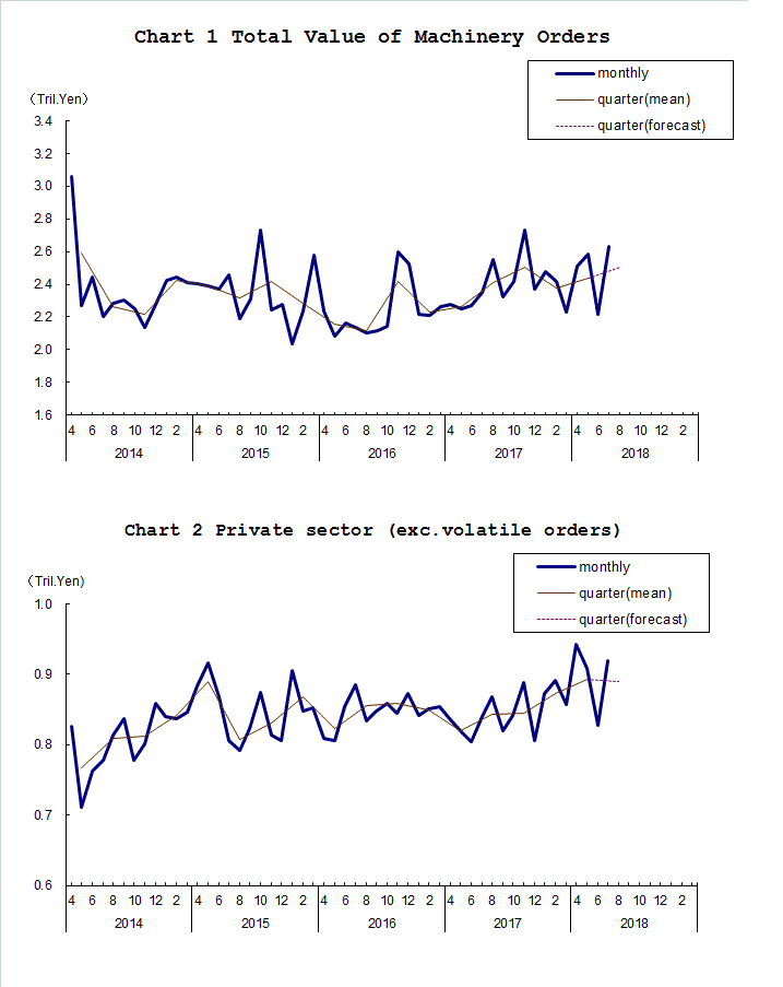
In Japan, private machinery orders, excluding volatile ones, rose 11.0% yoy in July, well above expectation of 5.8% yoy. Total machinery orders rose 18.8% yoy. The strong growth suggests that companies were keen to invest despite the threat of trade protectionism. And rising capex will likely add to economic growth. So far, trade war worries haven't materialized in economic data yet.

Also released, domestic CGPI rose 3.0% yoy in August, below expetation of 3.1% yoy.

White House top economic advisor Larry Kudlow said yesterday that communications with Beijing had "picked up a notch". He also confirmed that Treasury Secretary Steven Mnuchin had sent an invitation letter to senior Chinese officials to restart trade talks. Also, "there's some discussions and information that we've received that the top of the Chinese government wishes to pursue talks."

Kudlow also added that "most of us think it's better to talk than not to talk, and I think the Chinese government is willing to talk." And, if they come to the table in a serious way to generate some positive results, yes, of course. That's what we've been asking for months and months."

But he also cautioned that "I guarantee nothing."

[php_everywhere instance="1"]

There are some contrasting comments from Fed officials today.

Fed Governor Lael Brainard said that "with fiscal stimulus in the pipeline and financial conditions supportive of growth, the shorter-run neutral interest rate is likely to move up somewhat further, and it may well surpass the longer-run equilibrium rate for some period." And to her, gradual interest rate hikes are likely to be appropriate.

On the other hand, St. Louis Fed President James Bullard emphasized that "you can't just say, 'unemployment is 3.9 percent, obviously we have to raise rates'; or, 'growth is fast, obviously we have to raise rates.'" He noted that "I don't think that feedback to inflation is very strong to be able to make that argument."

The interest in cryptocurrencies is growing day by day and most people recognize them as a popular payment and investment method. Cryptocurrency is used to pay for goods and services, for additional earnings and for trading in the exchange market. More individuals and legal entities start using cryptocurrency.

Cryptocurrency is a digital currency protected by cryptographic technology. It has common features with a fiat currency, they are both used as a means of payment, can be transferred or exchanged. But cryptocurrency is decentralized and peer-to-peer, that means it can be traded anonymously.

Why are cryptocurrencies attractive?

• The creation of digital money is based on unique technologies.
• A trader can make a profit both on growth and on decrease. High volatility attracts many market participants to the market of cryptocurrencies.
• Crypto trading is available 24/7.
• The anonymity of information about the owner, transparency of all transactions and operations.
• Cryptocurrencies are protected by a cryptographic code, they are more reliable than fiat currencies.
• Limited emission – no inflation. Compared to fiat money, cryptocurrency can’t be generated in large quantities, that excludes inflation.
• Anyone can participate in mining, the process of issuing digital currencies, and get an appropriate reward for it.

Nowadays there are more than 1000 kinds of cryptocurrencies in the world. Cryptocurrencies are a new trend in the Internet trading. They are highly volatile, traders can make a significant profit on sharp price movements. Bitcoin, Ethereum, Litecoin, Ripple are promising and highly liquid trading instruments. Therefore, cryptocurrency trading has become increasingly popular among traders.

How to earn money while cryptocurrencies are losing their price?

Bitcoin as well as altcoins have become at least three times cheaper since the beginning of the year 2018. Now it’s hard even to return the investment for those who trade cryptocurrencies on crypto exchange. What if they could make profits from the price falls?

There is a ready answer to this; Forex Brokers offer Margin trading to their customers. It allows traders using Short selling strategy, allowing them to “go short”. It’s quite simple on Forex, you just need to open a sell order on a currency pair where, in your opinion, a quote currency is going to fall. After some time when the price are lower, you just have to close the order.

JustForex offers its clients to trade 13 cryptocurrency pairs including listed above cryptocurrencies. Crypto accounts from JustForex have a wide range of cryptocurrencies to trade, competitive spreads from 0, up to 1:3 leverage. Minimum deposit is not required.

In order to practice crypto trading at Forex, everyone can open a Demo account free of charge.

Gold rose on Wednesday after a posible meeting between the US and China to discuss trade was reported to be planned by US Treasury Sec Mnuchin. Trade war tensions have pressured the yellow metal making the US the most desired destination. Signs of goodwill form the US unlocked risk appetite and investors are taking gold to $1,207.

Gold is still sensitive to geopolitical factors. The economic calendar will bring inflation data in the US to the forefront. A higher inflation scenario could lock in two rates hikes for the U.S. Federal Reserve and keep gold in the current tight range. A solid CPI number in the States and the beating of the trade war drums are the worst case scenario for commodities this week.

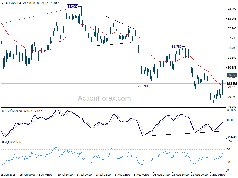
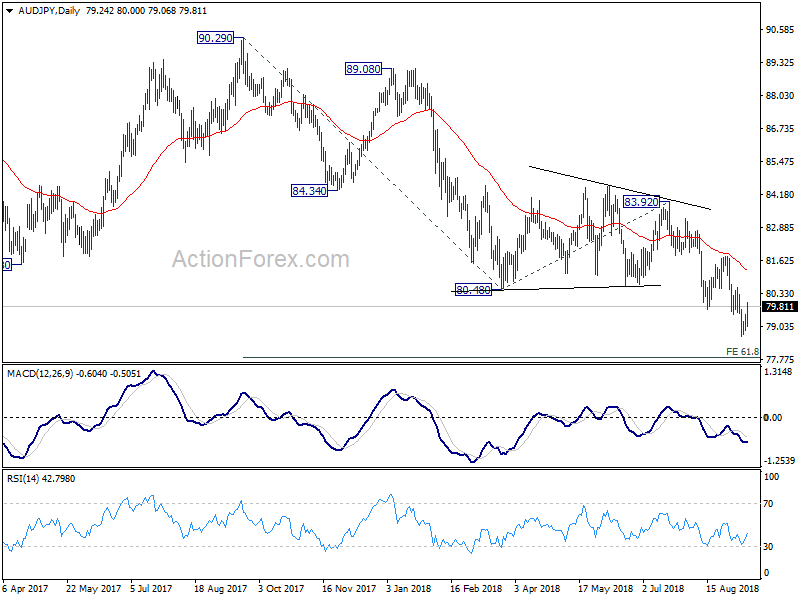
This is a follow up to our AUD/JPY short trade, entered at 80.25, stop at break even 80.25. Last updated in our weekly report.

AUD/JPY rebound strongly today on news that the US is trying to restart trade talk with China. And Trump intends to postpone the announcement of 25% tariffs on USD 200B in Chinese goods after that. Public hearing on the tariffs ended last week.

While the rebound is strong, our strategy is... don't panic. Firstly, at the time of writing, both he Treasury Department and Commerce Department declined to comment. So, it could be another piece of "fake news". Secondly, at the time of writing too, there is no follow through buying above 4 hour 55 EMA yet.

Technically, 4 hour technical doesn't look very promising, with bullish convergence condition in 4 hour MACD. But there is no confirmed reversal yet. Hence, we'd hold on to the short position, with stop unchanged at 80.25 (break even). But the chance for us to exit slightly above 61.8% projection of 90.29 to 80.48 from 83.92 at 77.85 has increased. We'll still not rigid exit there yet, as we'd like to give the cross a little breathing room on the news (real or fake).

And, after all, it's trading. Sometimes you win, sometimes you lose. Even if we're stopped out, it's not a loss!

We use an analytical framework we recently developed to inform our view of Fed policy going forward. We look for the FOMC to raise rates another 125 bps before it cuts rates at the end of 2020.

Is Fed Policy "Restrictive" Yet?

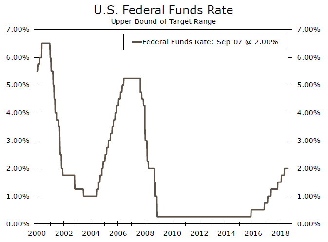
The Federal Reserve has raised its target range for the fed funds rate 175 bps since December 2015 (top chart). Naturally, there is interest in how much further the FOMC has to go and when the "terminal" fed funds rate will be reached. In a recent report, which is available upon request or on our website, we developed what we called "r-optimal" to help inform our views about the outlook for Fed policy. We employ the framework that was explained in that technical report to lay out our forecast of Fed policy through the end of 2020 in this non-technical report.

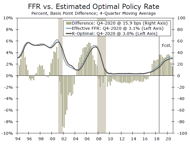
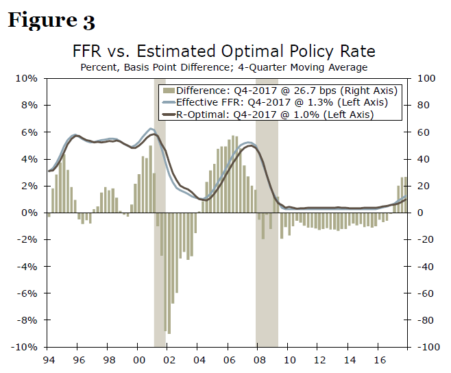
Our estimate of r-optimal along with the actual fed funds rate since 1994 is plotted in the middle chart. In prior tightening cycles, the FOMC has taken the fed funds rate about half a percentage point above r-optimal (middle chart). At that point, the Fed either subsequently backed off or the economy slid into recession. For example, the FOMC hiked the fed funds rate 275 bps between February 1994 and February 1995. But GDP growth slowed markedly in the first half of 1995, which prompted the Fed to subsequently reverse course. Between July 1995 and January 1996 the FOMC cut rates 50 bps. On two other occasions (2000 and 2006), the fed funds rate exceeded r-optimal by 50 bps or so on a four-quarter moving average basis and the economy subsequently entered recession.

As the middle chart also makes clear, r-optimal is not constant. As the economy strengthens and as the probability of "inflationary pressure" increases, r-optimal rises. Conversely, as economic growth weakens and the probability of "deflationary pressure" rises, r-optimal falls. The effective fed funds rate has been above r-optimal since early 2017, and we estimate that the difference between the two is nearly 40 bps at present.

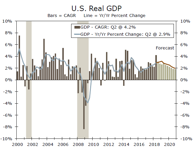
Our forecast looks for real GDP growth to remain solid in coming quarters (bottom chart) and for inflation to edge higher. This implies that r-optimal will rise from about 1 ½% at present to 2¾% by the end of next year. Consequently, the FOMC will need to raise its target range for the fed funds rate. Otherwise, monetary policy could end up being too accommodative, which would not be appropriate for an economy that is operating near full employment and is showing signs of rising inflationary pressures.

We look for the FOMC to hike rates in line with the trend increase in r-optimal. Specifically, we expect that the FOMC will raise its target range for the fed funds rate 25 bps at its September meeting and again at its December meeting. We also look for 75 bps of additional rate hikes next year, which would take the top end of its target range to 3.25% by Q3-2019. As growth slows in the second half of 2019 and into 2020, we expect that the Fed will remain on hold. However, we forecast that real GDP growth will slip below an annualized rate of 2.0% in the second half of 2020, which we believe will lead the FOMC to cut rates 25 bps at the end of 2020.

Executive Summary

A primary tool of monetary policy is the federal funds rate (FFR), which is the rate at which banks lend reserves to each other and functions as a key benchmark interest rate. The Federal Open Market Committee (FOMC), which is made up of Federal Reserve governors and District Bank presidents, sets a target range for the FFR based on policy goals. A higher FFR pushes up interest rates in the economy and therefore makes it more expensive to borrow, slowing down the economy. On the other hand, reducing the FFR makes it cheaper to borrow money, prompting consumers and businesses to spend more and boost the economy.

Determining the appropriate FFR to achieve policy goals is no easy task, as it relies on uncertain judgements about the current state of the economy and future prospects. In this report, we review common methods for estimating the appropriate target policy interest rate (we call this "r-optimal") and propose a new estimation framework. Our framework estimates r-optimal based on the probability of expansion/recession and inflationary/deflationary pressure, unlike traditional Taylor-type policy rules that calculate an optimal policy rate based on deviations of inflation from policymakers' objective and output from its "natural" or potential level. There are three major advantages of our methodology. First, it is forward-looking. Second, it does not use potential output as an explanatory variable, which is very difficult to estimate in real time.1 Finally, our methodology applies time-varying weights to inputs, which allows us to take into account the changing nature of risks in an evolving economy.

Traditional Methods: Taylor Rule and Modifications

One of the most widely known methods for guiding central bank interest rate policy is the Taylor rule, which was outlined by John B. Taylor in 1993.2 According to the Taylor rule, the appropriate federal funds rate should be determined as a function of inflation and the output gap (i.e., the difference between actual output and potential output in the economy). The output gap is commonly measured using deviations of unemployment from its natural rate. If inflation is higher than the Fed's target and/or when employment exceeds full employment, the FOMC should raise interest rates. Conversely, the FOMC should cut interest rates in periods of below-target inflation and high unemployment.

Traditionally, the Taylor rule uses backward-looking macroeconomic data as inputs, which is a main criticism since monetary policy is meant to be forward-looking.3 The FOMC regularly publishes forecasts of unemployment and inflation and estimates of its longer-run ("natural") values, which can be used in Taylor-type policy rules as an alternative. However, models are sensitive to the accuracy of estimates used as inputs. As pointed out by Federal Reserve Chair Powell (2018), real-time estimates of longer-run economic quantities are prone to error, since they cannot be directly observed. For instance, in retrospect, observers at the time significantly under-estimated the natural unemployment rate in the 1965 to 1980s period, but significantly over-estimated it in the 1990s.4

In addition, Taylor rule-type models usually apply fixed weights to input values. John Taylor's original 1993 paper, for instance, specifies a weight of 0.5 for the inflation and output gaps. The problem here is that fixed weights imply that the nature of risks remains constant over time, a strong assumption given that economies evolve. For example, the nature of inflation risk to the economic outlook has changed significantly over the past four decades, with a risk of high inflation in the 1980s giving way to a risk of deflation in recent years. Therefore, we argue that a time-varying weights approach is more effective to assess contemporary risks and design monetary policy accordingly.

Our Framework: A Probabilities-Based Approach

We estimate r-optimal based on the current level of the FFR and the future probabilities of expansion/recession and inflationary/deflationary pressure. This means that our model is forward-looking, as should be the case for monetary policy given the delay between a change in policy and its effect on the economy. In addition, our model does not rely on estimates of the natural rate of unemployment, which are difficult to make in real-time, as discussed by Powell in a recent speech at the Kansas City Fed's Economic Policy Symposium in Jackson Hole.5 Admittedly, estimating probabilities of recession and inflation is also prone to error. However, by using different inputs from traditional models, our framework adds to the data points that can be used by policymakers to guide interest rate policy.

Previously, we developed probit models to estimate the six-month and two-quarter ahead probabilities of inflationary/deflationary pressure and expansion/recession.6 The output of these models is shown in the figures below. In Figure 1, the shaded bars above the zero-line represent periods of inflationary pressure, which we characterize as periods in which PCE inflation exceeds 2.5%, while bars below the zero-line represent periods of deflationary pressure (i.e., periods in which PCE inflation is less than 1.5%). PCE inflation is in a range between 1.5% and 2.5% (i.e., "stable prices") in regions with no shaded bars. In simulated real-time analysis, our model has predicted all inflation outlook episodes accurately, and we therefore judge our model to be a reliable estimate of current and near-term inflation.

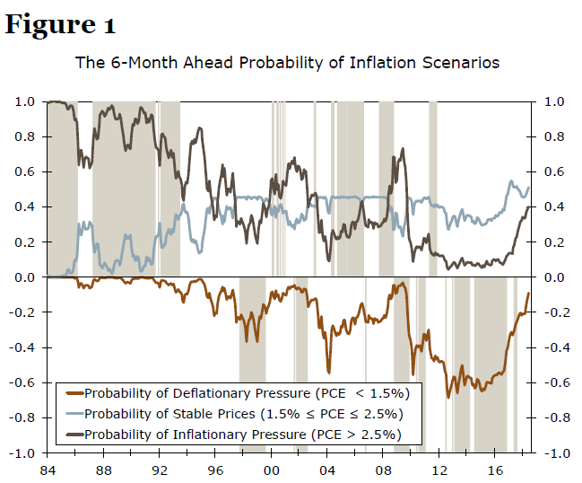
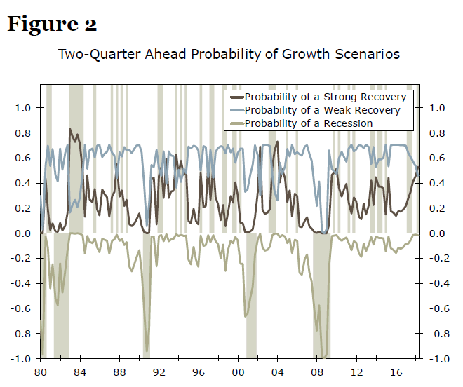
Figure 2 shows the probit model for probability of expansion/recession in the next two quarters. Here, the shaded bars below the zero-line represent recessions, the shaded bars above the zero-line represent strong recoveries (or expansions), and non-shaded gaps represent weak recoveries. Again, our model does a good job of predicting the three growth scenarios in simulated real-time analysis, which makes us comfortable using it as an input to estimating r-optimal.

Our model for r-optimal includes the probabilities of recession, stronger recovery, inflationary pressure and deflationary pressure as explanatory variables. We exclude the probabilities of stable prices and weak recovery, as these are used as the benchmark scenarios. Lastly, we include a one-quarter lag of the current nominal FFR as an explanatory variable, which allows us to incorporate the current monetary policy stance in the estimation process (since the future FFR depends on its current level). This follows a modification of the Taylor rule proposed by Clarida, Gali and Gertler (1999).7

We estimate the model using fixed weights for the entire time period of our analysis (1975-2018) as well as using time-varying weights. To calculate the time-varying weights, we estimate the model separately for three different sub-samples, which are determined based on the different growth/inflation/interest rate regimes during these periods.8 As discussed previously, using timevarying weights on our explanatory variables allows us to take into account the evolving nature of risks in the economy over time. This methodology also differentiates our framework from traditional Taylor-type policy rules that use fixed weights.

R-Optimal Estimation Results and Evaluation

Our estimation of r-optimal is shown in Figure 3. The green bars on the right axis show the deviations of the effective FFR from r-optimal. If the green bars are positive, this suggests that the effective FFR is above the optimal value. In that case, the FOMC may need to consider eventually reducing its target range for the FFR. Conversely, periods of negative green bars means that the effective FFR is below r-optimal, and that the FOMC may need to eventually raise the FFR target range. In a sister report to this one, we will walk through the implications of our estimate of roptimal for the path of monetary policy in coming years.9

Next, we compare the final results of our r-optimal model to several benchmarks to evaluate our results and their usefulness for guiding monetary policy. The main benchmark that we use is a Taylor-type policy rule developed by St. Louis Federal Reserve President James Bullard (2018).10 The explanatory variables in Bullard's model are his estimation of the natural real rate of interest, the deviation of unemployment from its natural rate (as estimated by the St. Louis Fed) and the deviation of inflation from the Fed's 2% target. Bullard estimates his model using two different sets of fixed weights, taken from Taylor (1993) and Taylor (1999). Based on the ranges of his inputs, Bullard's model gives a recommended policy rate in Q4-2017 of 8 bps to 161 bps using the first set of weights and 15 bps to 207 bps using the second set of weights. As an additional benchmark, we apply a Hodrick-Prescott (H-P) filter to the effective FFR, which produces an estimate of the trend FFR using purely statistical methods.

As shown in Table 1, our estimates of r-optimal and the three benchmarks that we use fall within overlapping ranges.11 However, our estimates are slightly higher than those in Bullard (2018). In addition, the ranges from our model are narrower than the ranges from Bullard (2018) and the H-P filter method. In particular, the estimated range produced from our time-varying weights model is smaller than from the other methods, including our estimation for r-optimal using the entire sample period. This is because the standard error for our model using the 2000-2018 sub-sample is only 0.34, compared to 0.90 for the entire sample period (since 1975).

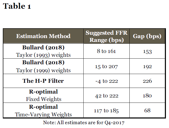
We argue that a narrower range of values for r-optimal makes our method more useful for guiding policymaking. Given that the FOMC typically moves rates only 25 bps at a time, the ranges estimated by Bullard (2018) for Q4-2017 would have allowed the FOMC to hike interest rates twice (as it actually did in H1-2018), while staying within the upper bound of his range, but also would have allowed the FOMC to cut interest rates twice without crossing below the lower bound of Bullard's estimated range. In contrast, our preferred estimate (r-optimal using time-varying weights) gives a range of only 68 bps, or a total of two possible 25 bps rate moves.

Comparing Sub-Sample Coefficients

In Table 2, we compare the estimated coefficients of our model when using the entire 1975-2018 sample period (fixed weights) versus sub-samples (time-varying weights). The sub-sample analysis allows us to examine whether different economic regimes are associated with different coefficient values, and thus how the nature of risks to the economic outlook has changed over time. We determined the dates of the sub-samples based on different growth/inflation/interest rate regimes.12 For example, the 1975-1989 period contains higher growth, inflation and interest rates relative to other periods. Meanwhile, the post-2000 period is associated with much slower economic growth, lower inflation and lower interest rates.

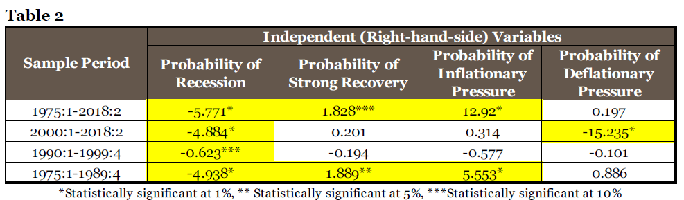
For the complete 1975-2018 sample period, the probabilities of recession, strong recovery and inflationary pressure are all statistically significant explanatory variables for the effective FFR (at the 10% confidence level, highlighted in yellow). If a variable is statistically significant, this suggests that it is useful for determining the appropriate policy rate (r-optimal). As would be expected, an increase in the probability of recession suggests a decrease in r-optimal (more accommodative monetary policy), while increases in the probability of a strong recovery and inflationary pressure lead to an increase in r-optimal (more restrictive monetary policy).

When the model is re-estimated on different subsamples, the statistically significant variables change, though their signs remain consistent. This suggests that different variables are more relevant to monetary policymaking during different periods, which makes sense within the historical context. For instance, in the most recent period (2000-2018), the only statistically significant variables are the probability of recession and the probability of deflationary pressure. This result is not surprising given the context of slow economic growth and low inflation.

The variability in the coefficient values (and their statistical significance) between the sub-sample estimations supports our hypothesis that risks to the economic outlook and their importance for policymaking evolve over time. Therefore, we conclude that time-varying weights are most appropriate to use in modelling a recommended policy interest rate. This is the methodology that we employ in our preferred estimate of r-optimal.

Conclusion

This report presents a new approach to estimate the optimal FFR. We believe that our framework adds to the current body of models for estimating a recommended policy rate and, therefore, provides a useful tool for policymakers to evaluate the current stance of monetary policy. In our follow-up report, we discuss our current estimation of r-optimal and implications for the path of the FFR over the next few years.

1 Jerome H. Powell. "Monetary Policy in a Changing Economy," (Changing Market Structure and Implications for Monetary Policy Symposium, Jackson Hole, WY, August 24, 2018).

2 John B. Taylor. "Discretion vs. Policy Rules in Practice." Carnegie-Rochester Conference Series on Public Policy 39, no. 1 (1993), 195-214.

3 Ben S. Bernanke. "Monetary Policy and the Housing Bubble," (Annual Meeting of the American Economic Association, Atlanta, GA, January 3, 2010).

4 Powell, "Monetary Policy in a Changing Economy," 2018.

5 Ibid.

6 See "Predicting the Probability of Inflation/Deflation: An Ordered Probit Approach" (February 17, 2014) and "Predicting the Probability of Recession and Strength of Recovery: An Ordered Probit Approach" (July 19, 2016). All Wells Fargo reports referenced herein are available upon request.

7 Richard Clarida, Jordi Gali & Mark Gertler. "The Science of Monetary Policy: A New Keynesian Perspective." Journal of Economic Literature 37, No. 4 (1999), 1661-1707.

8 The sub-samples we use are 1975-1989, 1990-1999 and 2000-2018.

9 See "How Much More is the Fed Likely to Tighten?" (September 12, 2018).

10 James Bullard. (2018). "R-star wars: the phantom menace," Business Economics 53, 60-65.

11 For comparison with Bullard (2018), all estimates are for Q4-2017. The ranges for our estimates of r-optimal and for the H-P filter estimate represent one standard deviation above and below the point estimate.

12 Another choice would be to divide the dataset into sub-samples according to business cycles. However, lengths of business cycles vary significantly from a range of 12 months (1980-1981 business cycle) to 120 months (1991-2001 business cycle). Some business cycles' shorter time span may affect the statistical accuracy of our results. Therefore, we divide data into sub-samples to represent different economic regimes and to avoid the problem of shorter time spans. Moreover, due to the shorter time span for the post-Great Recession period, we are using the post-2000 period to represent the most recent era.