Sample Category Title
Fed’s Williams: Policy well-positioned, unlikely to see further rate hikes
New York Fed President John Williams told CNBC overnight that current monetary policy is "well-positioned" and "restrictive" enough to help bring inflation down to target levels. He added that further rate hikes are unlikely, stating, "I don't see that as the likely case."
Williams highlighted that interest rates in the US will "eventually need to come down" based on data analysis, but the timing will depend on how effectively the Fed achieves its goals. He expects inflation to moderate in the second half of this year as the economy finds better balance and global inflationary pressures ease.
However, Williams emphasized, "Inflation is still above our 2% longer-run target, and I am very focused on ensuring we achieve both of our dual mandate goals."
Euro Suffers When ECB Announces the First Rate Cut of the Cycle
- ECB prepares to cut rates for the first time ahead of the Fed
- History points to strong possibility of back-to-back rate cuts
- Both the euro and German DAX tend to underperform on meeting day
The ECB is on the brink of announcing its first rate cut since March 2016 as the overall rhetoric from ECB officials leaves little doubt about next week’s rate decision, with even the most hawkish members of the Governing council acknowledging the need for rate cuts. This will be the ECB's first step to gradually unwind the aggressive tightening recorded during the 2022-2023 monetary policy cycle.
ECB to cut ahead of the Fed
If the ECB confirms expectations, next Thursday’s rate cut will mark the first time that the ECB will ease its monetary policy stance ahead of the Fed. Up to now, the Fed has always been dictating the start, the end, and the pace of any monetary policy cycle. However, with US inflation remaining quite sticky on the back of potent consumer spending, and the US Presidential elections being around the corner, Fed members’ hands are currently tied.
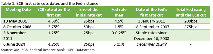
Table 1 below presents the initial rate cuts announced by the ECB during its three monetary policy easing cycles since 2000 along with the Fed’s stance at that time.
Back-to-back rate cuts?
Despite some positive news on the economic front from the recent PMI surveys, numerous ECB members appear supportive of another rate cut at the July meeting. Such an outcome will be closely examined in the behind-the-door discussions during the June meeting, with any likely decisions clearly contingent on the quarterly inflation projections presented by the ECB staff.
Interestingly, the ECB has, in the past, selected to ease in successive meetings. More specifically, in 2008, four consecutive rate cuts were announced, while in the 2011 easing cycle the ECB cut rates in two straight meetings before pausing to evaluate the situation.
Performance on the day of the rate cut announcement
Most ECB rate cuts are usually implied or even pre-announced in order to prepare the market and avoid an acute reaction. This time around, ECB members have been crystal clear about the outcome of next week’s gathering, allowing the market to run ahead of itself and to start pricing in a plethora of rate cuts in 2024 and 2025.
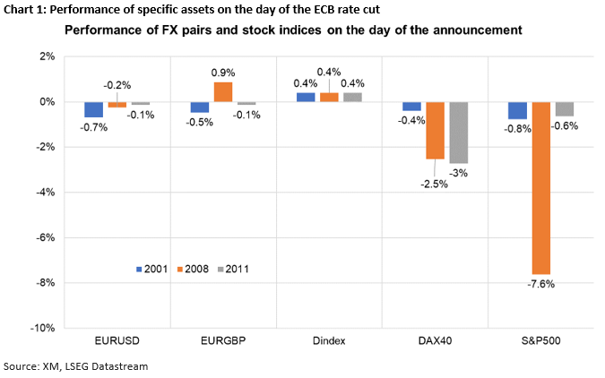
Despite the strong expectations, there is usually a market reaction on the day of the rate cut announcement. As seen in Chart 1 below, in the three respective dates presented earlier, euro/dollar tends to sell off by 0.1-0.7% as the market always tries to price a series of rate cuts, helping the dollar index rally in these three occasions. This euro underperformance can also be seen in the euro/pound pair.
Interestingly, the DAX 40 index exhibits a tendency to finish the rate cut announcement day significantly in the red, although these negative moves could be caused by the underperformance recorded in the S&P 500 index.
Market performance one week after the first rate cut
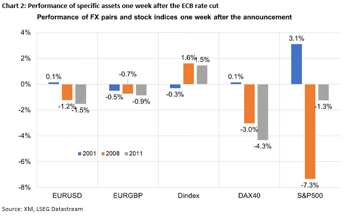
Chart 2 below shows the performance of specific FX pairs and stock indices one week after the first ECB rate cut is announced. The euro tends to remain under pressure, especially against the pound but less against the dollar. Similarly, the DAX 40 index shows a tendency for stronger losses as the market digests the new ECB outlook and prepares for the next rate cuts.
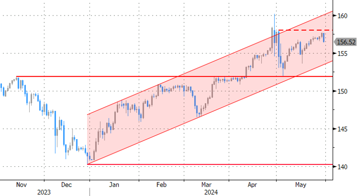
USD/JPY Stays Strong: Support Levels Hold Firm
Key Highlights
- USD/JPY started a downside correction from the 157.70 zone.
- A major bullish trend line is forming with support at 156.00 on the 4-hour chart.
- Gold prices are consolidating above the $2,320 support zone.
- Bitcoin price could aim for a move above the $70,000 level.
USD/JPY Technical Analysis
The US Dollar started a major increase above the 154.50 resistance against the Japanese Yen. USD/JPY traded toward 158.00 before the bears emerged.
Looking at the 4-hour chart, the pair started a downside correction and traded below 157.20. There was a move below the 23.6% Fib retracement level of the upward move from the 153.59 swing low to the 157.70 high.
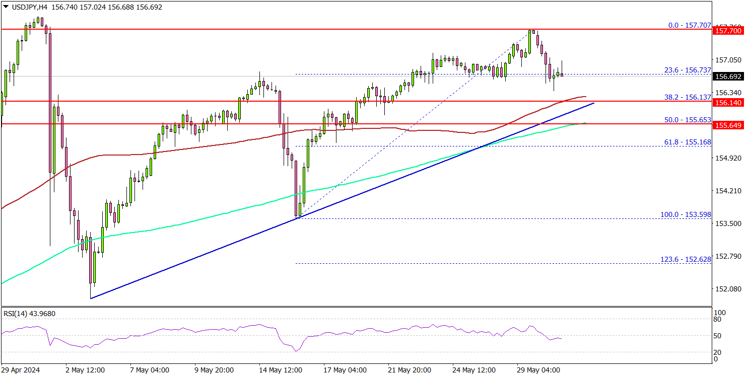
However, the pair is now holding gains above the 156.00 zone. There is also a major bullish trend line forming with support at 156.00 on the same chart.
The trend line is near the 38.2% Fib retracement level of the upward move from the 153.59 swing low to the 157.70 high and the 100 simple moving average (red, 4-hour). The main support is near the 155.65 level and the 200 simple moving average (green, 4-hour).
Any more losses might impact the current bullish trend. On the upside, immediate resistance is near the 157.20 zone. The first major resistance is near the 157.50 level.
A clear move above the 157.50 resistance might send it toward the 157.80 level. Any more gains might call for a move toward the 158.00 level in the near term.
Looking at Gold, the bulls are active near the $2,320 level and they might aim for a move toward the $2,400 level in the near term.
Economic Releases
- US Personal Income for April 2024 (MoM) - Forecast +0.3%, versus +0.5% previous.
- US Core Personal Consumption Expenditure for April 2024 (MoM) - Forecast +0.3%, versus +0.3% previous.
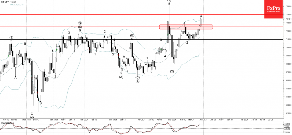
CHFJPY Wave Analysis
- CHFJPY broke key resistance level 172.50
- Likely to rise to resistance level 174.00
CHFJPY currency pair recently broke above the key resistance level 172.50, which has been repeatedly reversing the price from the end of April.
The breakout of the resistance level 172.50 should accelerate the active minor impulse wave 3 of the higher order impulse wave (3) from the start of May.
Given the clear daily uptrend and the continuation of the yen sales, CHFJPY currency pair can be expected to rise further to the next resistance level 174.00.
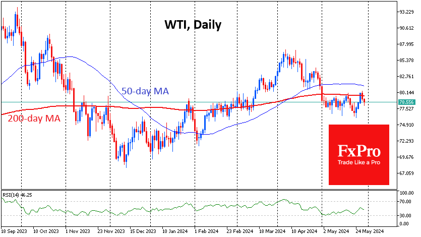
OPEC+ Meeting Could Switch Oil Regime
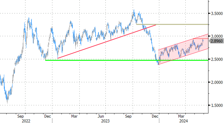
Oil declined for the second day in a row, reversing down from its 200-day moving average for the third time this month. An OPEC+ meeting is scheduled for this weekend with enough potential to break the tie.
Oil’s upward trend that started in December stopped in April with an impressive 12% correction. But it failed to develop, and throughout May, we saw fluctuations around the $78 average level with increasing amplitude.
Technically, the failure to develop a rise above the 200-day average is a sign that the bears are in control. The same is evidenced by the 50-day average above price and reversing downward during May.
The news media has been thickening the colours by pointing out the fall in discipline within OPEC+, which is producing well above quota, so the market is not creating an oil shortage and lower inventories as the cartel’s forecasts promise.
In 2014, Saudi Arabia, the leader of the cartel that provides the largest voluntary production cuts, had already surprised the world by suddenly expressing support for lifting the restrictions, which set off oil price wars.
But that strategy failed, eventually bringing the cartel to OPEC+, which includes members who agree on their production quotas but are officially in it, led by Russia.
So far, there is little sign that Saudi Arabia or Russia will return to the practice of oil wars. Nevertheless, for a rather fragile market, even a signal that no further cuts are expected and that the agreed quotas will be gradually raised could be a sufficient reason to sell off.
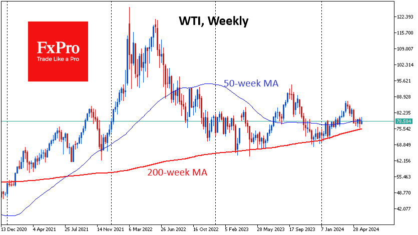
Special attention, in our view, should be paid to the support in the form of the 200-week moving average, which invariably triggered the cartel’s response. It is now nearly $75. A decisive decline below it will indicate a change in the market regime.
The bullish scenario assumes that the price’s proximity to the sensitive zone for the meeting will force OPEC+ to choose a tougher tone in its comments and promises, bringing oil back to growth. In this case, an important marker would be the ability to rise above $80.
ETHUSD Pulls Back from 2-Month High
- ETHUSD posts fresh 2-month high following ETF approval
- But sustains some losses as advance seems overstretched
- Momentum indicators ease from overbought conditions
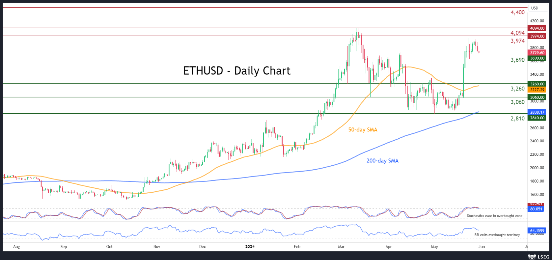
ETHUSD (Ethereum) has been on the rise after claiming the 50-day simple moving average (SMA) in mid-May. Moreover, the regulatory approval of spot-Ethereum ETFs in the US boosted the price to a fresh two-month peak of 3,974 before erasing some gains.
Should the latest weakness persist, the price could challenge 3,690, a region that has acted both as support and resistance in 2024. Lower, the bears’ attempts for further declines could cease at the March-April support of 3,260, which lies very close to the 50-day SMA. Slicing through that barrier, the pair might challenge the March bottom of 3,060.
On the flipside, if the bulls regain total control, the price could revisit its two-month peak of 3,974. A violation of that zone could pave the way for the 2024 high of 4,090, which is also a more than two-year high. Should that barricade fail, attention might shift to 4,400, a region that was frequently tested from October till December of 2021.
Overall, although ETHUSD stormed to a fresh two-month high supported by its individual developments, it seems that its rally is running out of juice. Hence, traders should not rule out another sell-the-fact type of reaction given what we have previously seen this year in the crypto sector.
Sunset Market Commentary
Markets
The two-day sell-off on core bond markets slightly went into reverse today. A downward revision to US Q1 price deflators (core PCE 3.6% Q/Q from 3.7%) and Q1 personal consumption (2% Q/Q from 2.5%) triggered the leap higher in which US Treasuries outperform German Bunds. Weekly jobless claims continue to hover near extremely low levels (219k from 216k) but didn’t have any market impact. US yields currently lose 4.2 bps to 5.7 bps with the belly of the curve outperforming the wings. Changes on the German curve were much more modest, varying between -1 bp to -2 bps. European data showed near consensus Spanish CPI (3.8% Y/Y for headline and 3% Y/Y for core) and an unexpected decline in April EMU unemployment rate (6.4% from 6.5%, lowest level since 1999). ECB members are already in their quiet period ahead of next week’s policy meeting. The blackout for the Fed starts this weekend with a potentially final significant appearance by NY Fed Williams at the Economic Club of New York later today. We especially look for views on the level of the neutral rate, once labelled the “phantom menace” by former St-Louis Fed governor Bullard. Heavyweight Fed governor Waller last week stressed that market perception on this theoretical equilibrium rate is too low and below levels where the Fed sees it (2.5%-3%). It’s one of the reasons why he thinks long term rates should be higher. An acknowledgement of a higher neutral in the June dot plot could serve as a new wake-up call to investors. Loss of interest rate support pulled the dollar away from first minor resistance levels. The trade-weighted dollar (DXY) failed to move beyond 105.12 (last week’s high) with return action to currently 104.77. EUR/USD similarly bounced off the 1.08-area to change hands at 1.0827. EUR/GBP holds dangerously close to the 0.85 support zone. The lack of BoE-speeches and UK eco data planned in coming days suggests that this bottom will hold for at least a little bit longer.
News & Views
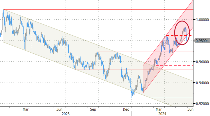
The economic barometer of the Swiss KOF Economic Institute unexpectedly softened in May from 101.9 to 100.3 (vs 102.1 expected). The Institute labelled the outcome as a muted momentum. The index this year only managed to stay very slightly above its medium-term average. The indicator bundles for manufacturing, financial and insurance services and foreign demand slowed down in May after having recorded positive developments in the previous month. Especially the manufacturing sector showed broad-based weakness. The indicators for private consumption and the construction industry cushioned the decline with increases. A separate data release from the Swiss State Secretariate of economic affairs, upwardly revised Q1 economic growth to 0.5% Q/Q, up from 0.3% in Q4 2023. Adjusted for the turnover of global sport organizations such as OIC, FIFA en UEFA, the GDP pace remained stable at 0.3% Q/Q. Growth was mainly driven by solid private consumption (+0.4%) and investment in equipment (+0.8%, a first rise after three negative quarters). Foreign trade negatively contributed to growth as strong imports (+2%), coincided with lackluster exports (goods -3.3%, services +1%). The Swiss franc rebounded sharply today, but this was mainly due to SNB Jordan signaling that the recent correction of the franc has gone far enough. EUR/CHF lost one big figure over the past two trading sessions, from 0.99 to 0.98.
Belgian CPI inflation rose in May by 0.37% M/M, leaving the Y/Y measure almost unchanged at 3.37%. Compared to April, the most significant price increases were registered for fruit (4.7%), clothes (1.3%), rents (0.6%), travels abroad and city trips (1.8%) and restaurants and cafés (0.5%). Motor fuels (-2.3%), electricity (-2.9%) and vegetables (-1.3%) had a decreasing effect on the index M/M. Compared to the same month last year, services inflation eased to 3.88% Y/Y from 4.93%. Food inflation increased slightly to 1% Y/Y from 0.25% in March and compared with a 17.02% peak in March 2023. Energy inflation continues to rise, from 9.19% to 11.17% Y/Y and accounts for 0.95 ppts in total inflation. The rise in inflation in recent months is due to the phase-out of the impact of the basic package for electricity and natural gas. Core inflation excluding prices of energy and unprocessed food, slowed to 2.8% Y/Y from 3.26% and 3.85% in April and March respectively. The first inflation estimate according to the European harmonized index of consumer prices (HICP flash estimate) for Belgium amounts 4.9% Y/Y.
Graphs
EUR/CHF: enough is enough for SNB Jordan
EUR/SEK: SEK profits slightly from Q1 GDP beat (+0.7% Q/Q) which was mainly driven by inventory build-up though
EU10y swap rate: previous YTD top holds, for now
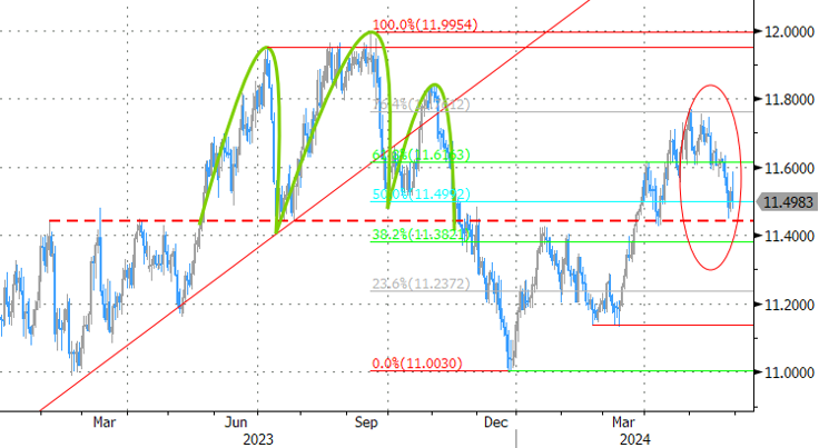
USD/JPY: Japenese MoF officials saved by today’s correction in lower core bond yields
US: Q1 GDP Revised Slightly Lower, But Details Show Domestic Economy Still Strong
The second estimate of first quarter real GDP growth was revised down 0.3 percentage points (pp) to 1.3% quarter-over-quarter (annualized) – bang-on the consensus forecast.
Looking under the hood, downward revisions to consumer spending, private inventory investment, and federal spending were partly offset by upward revisions to state & local government spending and fixed investment.
Consumer spending was downgraded to a 2.0% pace (previously 2.5%), largely due to a sharper pullback in durables spending (-4.1% vs. prior -1.2%). Non-residential investment was revised 0.4pp higher to 3.3%, thanks to a meaningful upgrade to intellectual property products (7.9% vs. prior 5.4%).
Federal spending was reported to have contracted by 0.7% (previously -0.2%), while state & local government spending rose by a slightly stronger 2.6% (previously 2.0%).
Net exports shaved 0.9pp from Q1 growth (unchanged from the prior estimate). However, the drag from net inventories is now reported to be slightly larger at 0.5pp (previously 0.4pp).
Real Gross Domestic Income (GDI) rose by 1.5% in the first quarter, a deceleration from Q4-2023's 3.6%. Corporate profits were a touch lower last quarter, falling 2.5% (annualized) or $21 billion after accounting for inventory valuation and capital consumption adjustments. However, the pullback was more than offset by a healthy 7.1% gain in personal income. The increase primarily reflected gains in compensation and personal current transfer receipts.
- The average of GDP and GDI, a supplemental estimate of domestic production, rose 1.4% in the first quarter – largely aligning to the pace of growth suggested by the expenditure GDP data.
Key Implications
The second estimate of first quarter GDP showed a slightly softer pace of economic expansion than previously reported. However, the overarching narrative has not changed. Even after accounting for the downward revisions, final sales to domestic purchasers (our best gauge of domestic activity) still advanced by a healthy 2.8% (previously 3.1%), and if not for a sizeable drag from net exports and inventories, first quarter growth would have come in at 2.6%.
April's personal income and spending data (released on Friday, May 31st) will give us the first snapshot on spending trends for Q2 and provide the revised monthly profile for Q1 PCE. While this morning's downward revision to spending implies less momentum coming into Q2, it is still tracking somewhere in the 2.5%-3% range. With the headwinds from first quarter growth abating, and the domestic economy still holding steady, Q2 GDP is tracking a trend-like pace of 2.3%.
EUR/USD Mid-Day Outlook
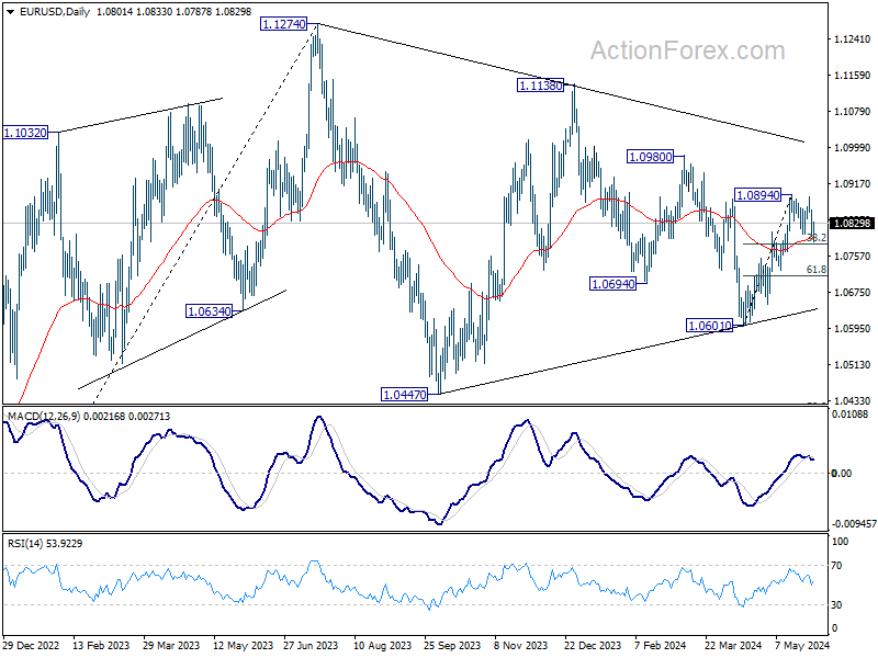
Daily Pivots: (S1) 1.0780; (P) 1.0821; (R1) 1.0842; More....
EUR/USD recovered after dipping to 1.0788 and intraday bias is turned neutral first. On the upside, firm break of 1.0894 will resume the rise from 1.0601 towards 1.0980 resistance next. However, sustained trading below 38.2% retracement of 1.0601 to 1.0894 at 1.0782 will argue that rebound from 1.0601 has completed. Deeper fall would be seen to 61.8% retracement at 1.0713.
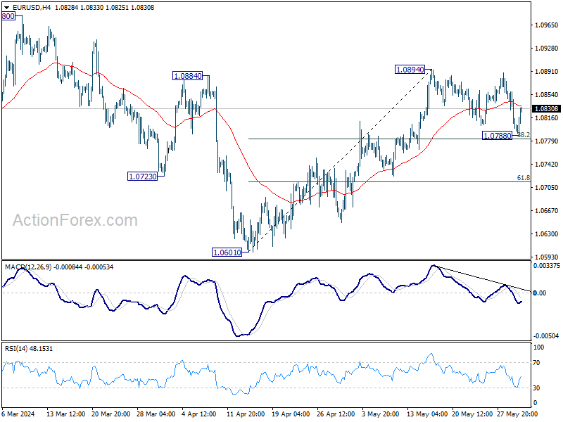
In the bigger picture, price actions from 1.1274 are viewed as a corrective pattern. Fall from 1.1138 is seen as the third leg and could have completed. Firm break of 1.1138 will argue that larger up trend from 0.9534 (2022 low) is ready to resume through 1.1274 high. On the downside, break of 1.0601 will extend the corrective pattern instead.